Lognormal Random Walk Model for Stock Prices Part 2

Lognormal Random Walk Model for Stock Prices (Part II)

A StockOpter White Paper

Note: This paper builds upon the Lognormal Random Walk Model for Stock prices Part I white paper.

Equation for a Future Price

Let:

• S₀ = the current price of the stock.
• S_t = the price of the stock t years from now.
• r = the expected continuously-compounded annualized increase in stock price.
• t = the time in years from now to the future date.
• s = volatility of the stock price.
• z = the number of standard deviations by which the ln of the stock price t years from now deviates from its mean. Since the ln of the stock price t years from now is assumed to be normally distributed, z is normally distributed with mean 0 and standard deviation 1.

What one should use for r depends on the context in which the calculation is being done. For the Black-Scholes model it is the risk-free rate. It is assumed for the Black-Scholes model that the stock does not pay dividends; paying dividends reduces a stock’s expected increase in price. For discussion of the Black-Scholes model, including modifications for stocks that pay dividends, there is a detailed white paper in the StockOpter University.

Investors in stocks expect the overall return on the stock, including both price appreciation and dividends, to be more than the risk-free rate to compensate them for the risk that they bear. This difference is called the risk premium. It can be ignored in the Black-Scholes model because doing so leads to two different errors that cancel one another. For purposes of the actual probability distribution of the future price, however, one should use a value of r that includes the effects of dividends if the stock pays dividends and of the risk premium.

In principle this includes Value at Risk (VaR) calculations. However, for an industry-standard one-day VaR calculation, the effect of r will be negligible compared to the effect of volatility. The effect of r will still be much smaller than the effect of volatility for StockOpter.com’s one-month VaR calculations, and as a result the simplifying assumption is made for those calculations that the risk premium is zero.

The volatility, s, is the standard deviation of the possible one-year changes in the ln of the price. It happens to also be the standard deviation of the ln’s of the possible prices one year from now, and also the standard deviation of the difference in ln between the possible prices one year from now and the expected price one year from now. This is due to the fact that the standard deviation of a set of numbers is the same as that of another set of numbers obtained by subtracting a constant from each of the numbers in the first set.

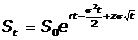
The price t years from now given the price today is given by

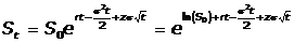
Taking the ln of each side of the equation gives

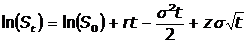
Thus, ln(S₁) is normally distributed with mean ln(S₀) + rt – s²t/2 and standard deviation s times the square root of t.

It makes sense that the expression for the mean would start from the value today, and include expected growth, but the ‑s²t/2 term calls for some explanation. The mean of the lognormal distribution of the price t years from now is given by

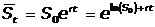
Thus, the point in the normal distribution of ln(S_t) that corresponds to the mean of the lognormal distribution of S_t is ln(S₀) + rt. However:

• The median (the 50^th percentile) of a lognormal distribution must be less than its mean, due to the large contribution to the mean of the small number of very high values (see the first graph in the Part I materials).
• The median of a normal distribution obtained from a lognormal distribution must be the ln of the median of the lognormal distribution, since the points are transformed one-for-one. Put another way, if the probability that x is less than A is 50%, then the probability that ln(x) is less than ln(A) must also be 50%.
• The mean of a normal distribution is the same as its median, due to the distribution being symmetrical.

Thus, the mean of a normal distribution must be less than the point corresponding to the mean of the corresponding lognormal distribution. The amount by which it is less is s²t/2 in this case. Why it is this particular amount is beyond the scope of this document.

As for the standard deviation of the distribution, s times the square root of t, s is the standard deviation of the ln of the price one year from now. It should make sense that the standard deviation will be less than this if t is less than one year, and more than this if t is more than one year. However, why the square root of t rather than t?

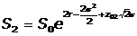
Consider the price two years from now arising from consecutive one-year changes. Let the subscripts 0, 1, and 2 stand for now, 1 year from now, and 2 years from now, respectively. Since the mathematics are the same for both of the one-year changes, and t for each change is 1,

z₀₁s + z₁₂s represents the sum of the year 1 deviation from its expected ln and the year two deviation from its expected ln. These are independent, since we are assuming a random walk. s is the standard deviation of each one year change. When the components of a sum are independent, the variance of the sum is the sum of the variances. Variance is the square of standard deviation. Thus, the standard deviation of the two year change is

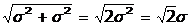
Thus,

Since 2 is the overall number of years that we are considering, We can generalize the above result as

which is our original equation.

The result that the standard deviation of the distribution is the annualized volatility times the length of the time interval in years is very important. Obviously it is important in the above equation, but in addition it allows us to calculate standard deviations of daily, or weekly, or monthly, etc., changes in ln, and then convert the result to an annualized historical volatility by dividing the result by the square root of the length of the time interval measured in years. The actual changes used are typically day-to-day changes.

The above derivation of the equation for a 2-year change in price from the equations for consecutive 1-year changes in price illustrates another important point about the lognormal random walk model for stock prices. That point is that if one models the change for a time period as taking place in a single step or taking place in several smaller steps one gets the same answer. Thus, one does not need to model smaller steps. You may recall from the Part I material that this is not the case for percent changes; for percent changes the results depend on how finely one has broken down the time intervals.

Confidence Bounds and Confidence Intervals

Since we are assuming that the possible values of the ln of the price at time t are normally distributed, where z is the number of standard deviations from the mean, we can use the properties of the standardized normal distribution to create confidence bounds and the like. For example, the 5^th percentile of the standardized normal distribution is -1.645 standard deviations, so substituting -1.645 for z in the above equation for P_t will give us the 5^th percentile of the possible prices at time t. Similarly, we can calculate the 95^th percentile of the possible prices at time t by using z = +1.645. The range between the two resulting values will be a 90% confidence interval, since there is a 5% chance that the realized price will be less than the lower bound price (the 5^th percentile price) and a 5% chance that the realized price will be greater than the upper bound price (the 95^th percentile price).

StockOpter.com makes use of these properties in its Value at Risk (VaR) calculations.

‍